2/4 Object:
- expand your portfolio optimization toolkit with risk measures such as Value at Risk (VaR) and Conditional Value at Risk (CVaR)
- use specialized Python libraries including pandas, scipy, and pypfopt.
- how to mitigate risk exposure using the Black-Scholes model to hedge an options portfolio.
Measuring Risk
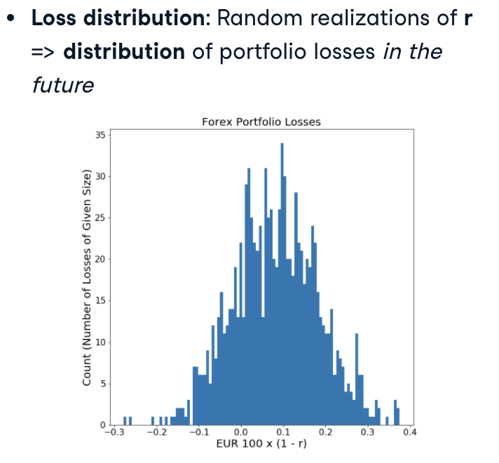
The Loss Distribution
Forex example:
EUR and USD (exchange rate is r)
r EUR = 1 USD
Loss = EUR 100 x (1-r)
random realization of r => distribution of portfolio losses in the future
Maximum loss
What’s the max loss of a portforlio?
Losses cannot be bounded with 100% certainty
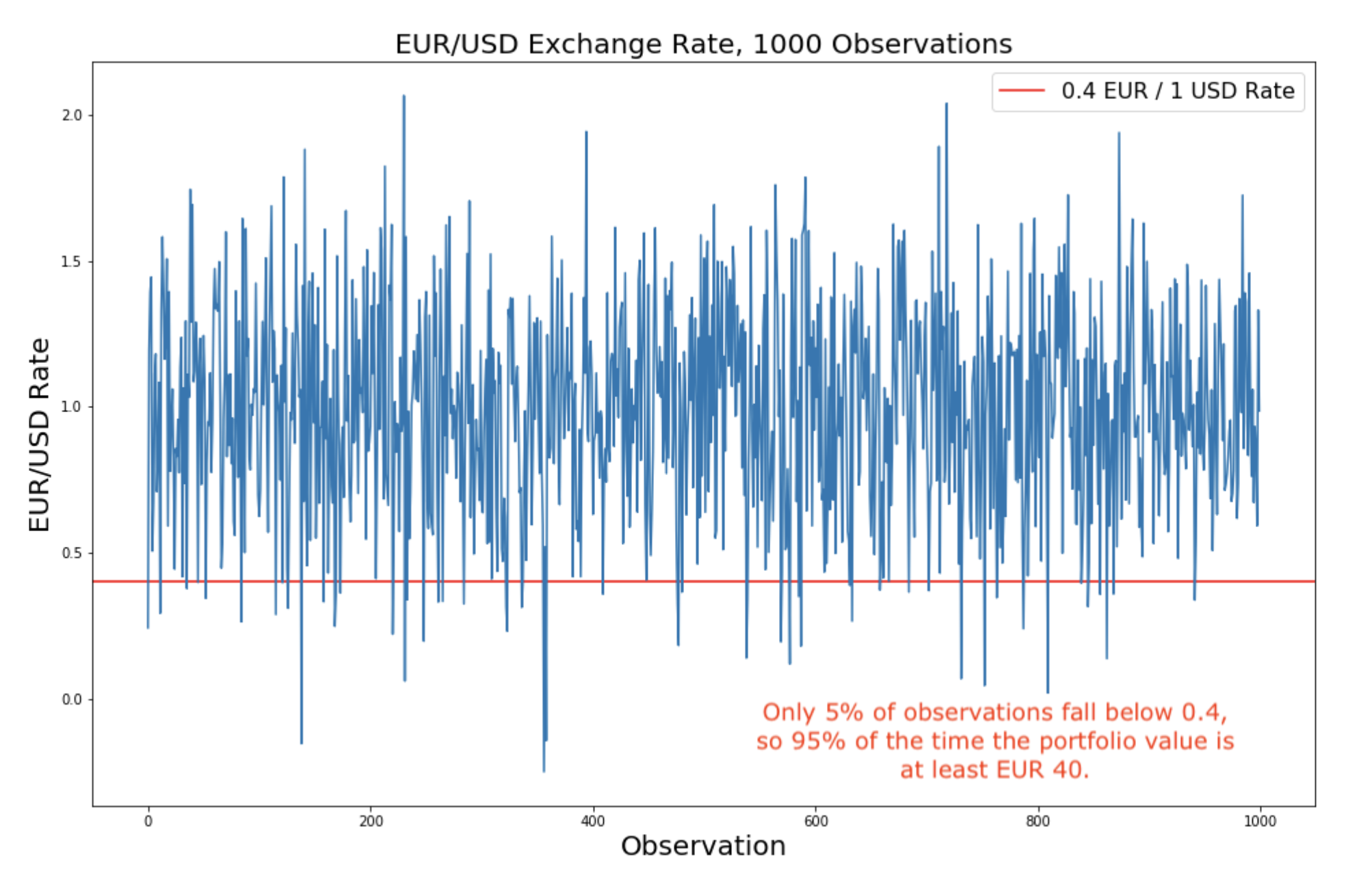
Confidence level: replace 100% certainty with likelyhood of upper bound
Can express questions like “what’s the maximum loss that would take place 95% of the time?”
- here the confidence level is 95%
Value at risk (VaR)
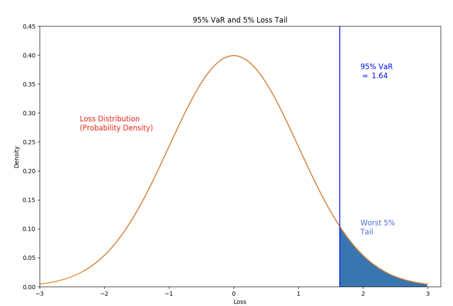
VaR(风险价值): statistic measuring maximum portfolio loss at a particular confidence level
某一置信度下的最大损失
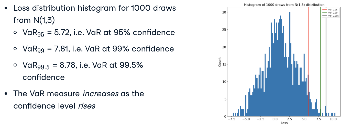
Typical confidence levels: 95%, 99%, and 99.5% (usually represented as decimals)

Forex example:
Conditional Value at Risk (CVaR)
CVaR(条件风险价值): measures expected loss given a minimum loss equal to the VaR. It equals expected value of the tail of the loss distribution
VaR的一个问题是他不考虑超过该置信度后的损失情况, 而CVaR表示投资组合的损失超过某个给定VaR值的条件下,该投资组合的平均损失值。

Deriving the VaR
- Specify the confidence level (e.g. 95%, 0.95)
- Creat a Series of
lossobservations - Compute
loss.quantile()at specified confidence level - VaR = computed
.quantile()at desired confidence level
1 | loss = pd.Series(observations) |
If we know losses are distributed according to a statistical distribution like the Normal distribution, we can also use the “.ppf()”, or percent point function, to find the VaR.
—> scipy.stats loss distribution: percent point function .ppf() can also be used.
Deriving the CVaR
- Specify the confidence level (e.g. 95%, 0.95)
- Creat or use sample from loss distribution
- Compute VaR at a specified confidence level
- Compute CVaR as expected loss (Normal distribution:
scipy.stats.norm.expected()does this)
1 | losses = pd.Series(scipy.stats.norm.rvs(size = 1000) |
Visulizing the VaR

*N(mean, variance) stands for normal distribution
Excercises
VaR for the Normal distribution
To get accustomed to the Value at Risk (VaR) measure, it helps to apply it to a known distribution. The Normal (or Gaussian) distribution is especially appealing as it 1) has an analytically simple form, and 2) represents a wide variety of empirical phenomena. For this exercise you’ll assume that the loss of a portfolio is normally distributed, i.e., the higher the value drawn from the distribution, the higher the loss.
1 | # Create the VaR measure at the 95% confidence level using norm.ppf() |
Comparing CVaR and VaR
The conditional value at risk (CVaR), or expected shortfall (ES), asks what the average loss will be, conditional upon losses exceeding some threshold at a certain confidence level. It uses VaR as a point of departure, but contains more information because it takes into consideration the tail of the loss distribution.1
2
3
4
5
6
7
8
9
10
11
12
13
14
15# Compute the mean and variance of the portfolio returns
pm = portfolio_losses.mean()
ps = portfolio_losses.std()
# Compute the 95% VaR using the .ppf()
VaR_95 = norm.ppf(0.95, loc = pm, scale = ps)
# Compute the expected tail loss and the CVaR in the worst 5% of cases
tail_loss = norm.expect(lambda x: x, loc = pm, scale = ps, lb = VaR_95)
CVaR_95 = (1 / (1 - 0.95)) * tail_loss
# Plot the normal distribution histogram and add lines for the VaR and CVaR
plt.hist(norm.rvs(size = 100000, loc = pm, scale = ps), bins = 100)
plt.axvline(x = VaR_95, c='r', label = "VaR, 95% confidence level")
plt.axvline(x = CVaR_95, c='g', label = "CVaR, worst 5% of outcomes")
plt.legend(); plt.show()
Risk exposure and loss
Deciding between options
- Chances of negaticve shock: probability of loss
- Loss associated with shock: amount or conditional amount (e.g. VaR, CVaR)
- Desire to avoid shock: Risk tolerance
Risk exposure and VaR
Risk exposure = probability of loss x loss measure
Loss measure: e.g. VaR
loss distribution:
normal distribution: good for large number of samples
students’ t distribution: good for small number of samples
Risk appetite
- Insurance is a way to pay a fixed value to avoid an uncertain outcome, which is risk-averse behavior.
risk averse (or risk avoiding) - if they would accept a certain payment (certainty equivalent) of less than $50 (for example, $40), rather than taking the gamble and possibly receiving nothing.
risk neutral – if they are indifferent between the bet and a certain $50 payment.
degrees of freedom (df)
number of independent observations
- Small df: “fat tailed” T distribution
- Large df: Normal distribution
Exercises
VaR and risk exposure
1 | # Import the Student's t-distribution |
CVaR and risk exposure
1 | # Fit the Student's t distribution to crisis losses |
结果为0.3380538488604617
Risk management with VaR and CVaR
Incorporating VaR into MPT
Mordern Portfolio Theory (MPT): “mean-variance” optimization
- Highest expected return
- Risk level (volatility) is given
- Objective function: expected return
VaR/CVaR: measure risk over distribution of loss
Adapt MPT to optimize over loss distribution vs. expected return
A new objective: minimize CVaR
change objective of portfolio optimization
- mean-variance objective: maximize expected mean return
- CVaR objective: minimize expected conditional loss at a given confidence level
—> Optimization: portfolio weights minimizing CVaR
—> find the lowest expected loss in worst (1-confidence) of possible outcomes
在给定的置信度下,可能出现的结果中,达到最低的损失
CVaR minimization using PyPortfolioOpt
- Create an
EfficientFrontierobject with an efficient covariance matrixe_cov - Import built-in objective function that minimizes CVaR,
negative_cvar()frompypopt.objective_functionsmodule - Comput optimal portfolio weights using
.custom_objective()method
(Arguements of.negative_cvar()added to.custom_objective).
1 | ef = pypopt.objective_frontier.EfficientFrontier(None, e_cov) |
Negative CVaR?
Seek minimum CVaR portfolio at given significance level 1-alpha
Same as finding portfolio that maximizes returns in worst 1-alpha cases
Question: expect objective function to return positive number, or negative?
Optimization can be either:
- maximize someting or
- minimize the negative of someting
PyPortfolioOpt solver: minimizes by default
- so objective function needs to be negative of CVaR returns
- Give same answer as minimizing CVaR losses
Term “negative CVaR” is a misnormer: CVaR is an expected loss
Mean-variance vs. CVaR risk management
Mean-variance risk management: minimize volatility
- We compute the minimum volatility portfolio weights in the usual fashion, by creating an EfficientFrontier instance and using the ‘min volatility’ method.
CVaR risk management: minimize negative CVaR - The CVaR-minimizing portfolio is created using the ‘custom objective’ and ‘negative cvar’ methods. The result is a roughly equally-weighted portfolio.
- This creates more volatility than the minimum volatility mean-variance portfolio, but with the benefit that the worst 5% cases of loss are minimized.
Excercies
VaR from a fitted distribution
Minimizing CVaR requires calculating the VaR at a confidence level, say 95%. Previously you derived the VaR as a quantile from a Normal (or Gaussian) distribution, but minimizing the CVaR more generally requires computing the quantile from a distribution that best fits the data.
1 | # Visualize the fitted distribution with a plot |
Minimizing CVaR
1 | # Import the EfficientFrontier class |
结果1
{'Citibank': 0.24991481239515553, 'Morgan Stanley': 0.2497894497565988, 'Goldman Sachs': 0.25013519444333526, 'J.P. Morgan': 0.2501605434049105}
CVaR risk management and the crisis
Derive the 95% CVaR-minimizing portfolio for 2005-2006, 2007-2008, and 2009-2010.1
2
3
4
5
6
7
8
9
10# Initialize the dictionary of optimal weights
optimal_weights_dict = {}
# Find and display the CVaR-minimizing portfolio weights at the default 95% confidence level
for x in ['before', 'during', 'after']:
optimal_weights_dict[x] = ef_dict[x].custom_objective(negative_cvar, returns_dict[x])
# Compare the CVaR-minimizing weights to the minimum volatility weights for the 'before' epoch
print("CVaR:\n", pd.DataFrame.from_dict(optimal_weights_dict['before']), "\n")
print("Min Vol:\n", pd.DataFrame.from_dict(min_vol_dict['before']), "\n")
结果1
2
3
4
5
6
7
8
9
10
11
12
13CVaR:
Weight
Citibank 0.248754
Morgan Stanley 0.249111
Goldman Sachs 0.250973
J.P. Morgan 0.251162
Min Vol:
Weight
Citibank 0.655621
Morgan Stanley 0.059033
Goldman Sachs 0.029725
J.P. Morgan 0.255621
Portfolio hedging: offsetting risk
Portfolio statbility
VaR/CVaR: potential portfolio loss for given confidence level
Portfolio optimization: “best” portfolio weights
- But volatility is still presents!
Institutional investors: stability of portforlio against volatile changes - pension funds: c. USD 20 trillion
Example: raning days and sunny days
Investors portfolio: sunglasses company
- Risk factor: weather (rain)
- More rain -> lower company value
- Lower campany value -> lower stock price
- lower stock price -> lower portfolio value
Second opportunity: umbrella company
- more rain -> more value
Portfolio: sunglasses & unbrella, more stable —> risk reduced
—-> Hedging: offset volatility with another asset
Hudging instrumentes: options (期权)
derivative hedging strategies (衍生对冲策略)
Hedging is often performed using derivatives to offset a risky asset position.
One of the most basic derivatives is the European option.
- A European ‘call’ option gives the holder the right (but not the obligation) to _purchase_ a stock for a fixed price X at a particular time M.
- A European ‘put’ option gives the holder the right (but not the obligation) to _sell_ a stock for a fixed price X at a particular time M.
The stock is called the ‘underlying’ of the option. The market price of the underlying is called the ‘spot’ price ‘S’. The fixed price is called the ’strike’ price ‘X’ and the time ‘M’ is the ‘maturity’.
Exercises
Black-Scholes options pricing
Black-Scholes 期权定价模型1
2
3
4
5
6
7
8
9
10
11
12
13
14# Compute the volatility as the annualized standard deviation of IBM returns
sigma = np.sqrt(252) * IBM_returns.std()
# Compute the Black-Scholes option price for this volatility
value_s = black_scholes(S = 90, X = 80, T = 0.5, r = 0.02,
sigma = sigma, option_type = "call")
# Compute the Black-Scholes option price for twice the volatility
value_2s = black_scholes(S = 90, X = 80, T = 0.5, r = 0.02,
sigma = 2*sigma, option_type = "call")
# Display and compare both values
print("Option value for sigma: ", value_s, "\n",
"Option value for 2 * sigma: ", value_2s)
结果1
2Option value for sigma: 12.129167513536352
Option value for 2 * sigma: 16.24149623118327
Options pricing and the underlying asset
1 | # Select the first 100 observations of IBM data |
Using options for hedging
1 | # Compute the annualized standard deviation of `IBM` returns |
结果为0.00459428051019628