3/4 objectives:
- estimate risk measures using parametric estimation and historical real-world data.
- discover how Monte Carlo simulation can help you predict uncertainty.
- learn how the global financial crisis signaled that randomness itself was changing, by understanding structural breaks and how to identify them.
Parameter Estimation
A class of distribution
theta: the vector of unknown parameters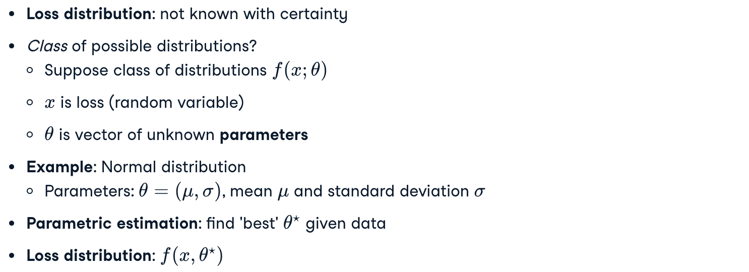
Fitting a distribution
Fit distribution according to error-minimizing criteria
- Example:
scipy.stats.norm.fit(), fitting Normal distribution to data - Result: optimally fitted mean and standard deviation
Advantages:
- Visualize difference between data and estimate using histogram
- Provide goodness-of-fit test
Goodness of fit

norm: too wild
t: good, taller’ and ‘narrower’.
This means that the degrees of freedom of the T distribution, which is the number of independent observations, is estimated to be low.
Although the T distribution provides a good fit, the data is still not quite right. In particular, the histogram is not symmetrical: it’s a bit lopsided.
Skewness (偏度/偏态、偏态系数)
Skewness: degree to which data is non-symmetrically distributed
是统计数据分布非对称程度的数字特征
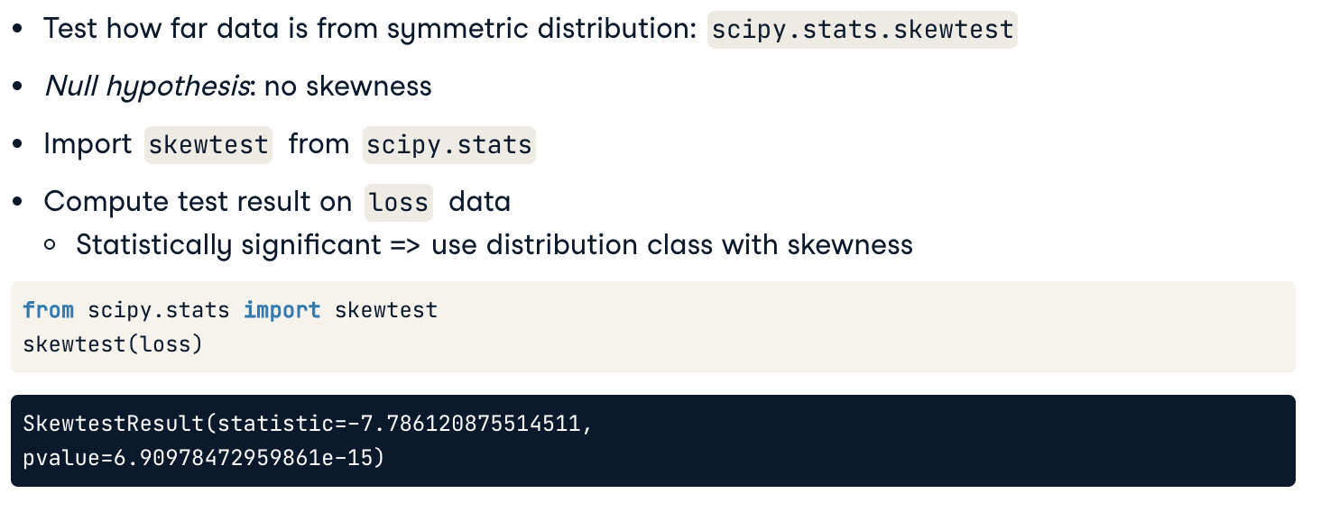
We can test for skewness in the data by seeing how far data are from being symmetric. In Python we test for skewness using ‘skewtest’ from ‘scipy.stats’. The null hypothesis is that there is no skewness, indicating that a symmetric distribution is appropriate. After importing the test, it is applied to the loss data. The results indicate both the test statistic value and its significance level. In our example, a test statistic of -7.78 has a more than 99.9% confidence level, showing that the data has statistically significant skewness. Parametric estimation using a Skewed Normal distribution might then be appropriate.
Exercises
Parameter estimation: Normal
1 | # Import the Normal distribution and skewness test from scipy.stats |
结果1
2VaR_95, Normal distribution: 0.07376954007991526
Anderson-Darling test result: AndersonResult(statistic=30.302775165424237, critical_values=array([0.573, 0.653, 0.783, 0.913, 1.086]), significance_level=array([15. , 10. , 5. , 2.5, 1. ]))
Parameter estimation: Skewed Normal
1 | # Import the skew-normal distribution and skewness test from scipy.stats |
结果1
2Skewtest result: SkewtestResult(statistic=-12.561846503056646, pvalue=3.4225103594408506e-36)
VaR_95 from skew-normal: 0.06759217691716421
Historical and Monte Carlo Simulation
Historical simulation in Python
Historical simulation: use past to predict future
VaR: start with returns in assets_returns
Compute portfolio_returns using portforlio weights
Convert portfolio_returns into losses
VaR: compute np.quantile() for losses at a confidence level
Assume future distribution of losses is exactly the same as past (which may not be true)
1 | weights = [0.25, 0.25, 0.25, 0.25] |
Monte Carlo Simulation in Python
Monte Carlo Simulation: A powerful combination of parametric estimation and historical simulation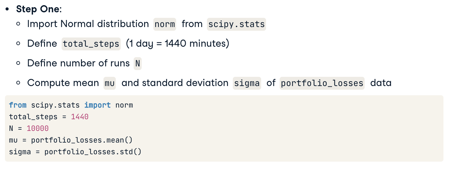
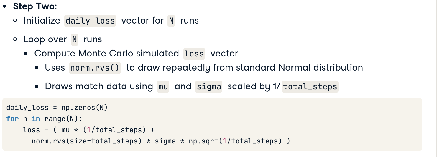
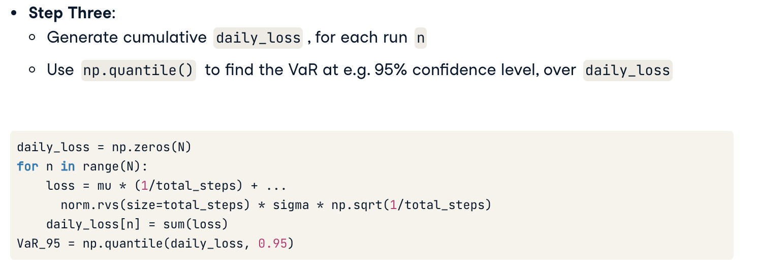
Simulating asset returns
A more thorough (and common) approach is to simulate the returns for the individual assets in a portfolio, rather than just the portfolio’s total return.
This allows greater realism as each risk factor can contribute their own sample path.
In addition, risk factors can be correlated: the covariance matrix e_cov can be used to compute asset returns in the simulation procedure.
Exercises
Historical simulation
Historical simulation of VaR assumes that the distribution of historical losses is the same as the distribution of future losses. We’ll test if this is true for our investment bank portfolio by comparing the 95% VaR from 2005 - 2006 to the 95% VaR from 2007 - 2009.
1 | # Create portfolio returns for the two sub-periods using the list of asset returns |
结果1
VaR_95, 2005-2006: 0.014687184472834514 ; VaR_95, 2007-2009: 0.05790574066814192
Monte Carlo Simulation
1 | # Initialize daily cumulative loss for the assets, across N runs |
结果1
Monte Carlo VaR_95 estimate: 0.0032448493079297045
Structural breaks
在计量经济学和统计学中,结构性折断是回归模型参数随时间的意外变化,通常会导致巨大的预测误差和模型的不可靠性。
Risk and distribution
Risk management toolkit:
- Risk mitigation: MPT
- Risk measurement: VaR, CVaR
Risk: dispersion, volatility
- Variance (standard deviation) as risk definition
Connection bewteen _risk_ and _distribution of risk factors_ as random variables
Stationarty (平稳性)
Assumption: distribution is the same over time
Unchanging distribution = stationary
Global financial crisis period efficient frontier —> not stationary
Estimation techniques require stationarity:
- Historical: unknown stationary distribution from past data
- Parametric: assumed stationary distribution class
- Monte Carlo: assumed stationary distribution for random draws
Structural breaks
If we knew that the distribution was changing over time, and we knew when distribution changes occur, then we could estimate our risk measures only during sub-periods when the distribution didn’t change.
In other words, distributions would be stationary only within certain sub-periods of the data.
Structural breaks: points of change
— change in “trend” of average and/or volatility of data
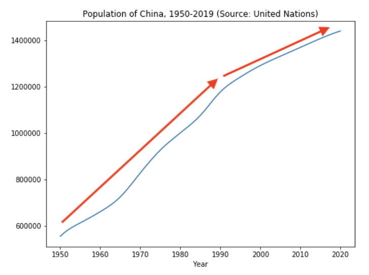
Example: China’s population growth
As an example of a structural break, let’s examine the population growth rate of China from 1950 to 2019. We can see that the growth is relatively linear over this period…
…but around 1990 the growth rate slows down. This indicates that there may be a structural break around 1990.
In other words, the underlying distribution of net population gains (births minus deaths) changed, causing there to be fewer net gains from 1990 onwards. Some reasons for such a change could be changes in government policy, changes in living standards, and other micro- and macro-level factors.
The Chow test
Previous example: A visual examination is useful to identify structural breaks.
the “Chow Test”: statistical measurement, which asks if the data support a structural break at a given break point of time, for a given linear risk factor model.
Null hypothesis: no structural break.
In the test, 3 ordinary least squares (OLS) regressions are performed:
- one for the entire period,
- two for before and after the break point.
The sum-of-squared residuals are then collected, and the Chow test statistic is created. The statistic is distributed as an “F”-distribution statistic.
The Chow test in Python
Let’s use the Chow test to see if there was a structural break somewhere around 1990 in China’s population growth. We’ll use a very simple “factor model” where log-population is regressed against year.
Step1: OLS regression of the whole period
An OLS regression over the 1950 - 2019 period, regressing the natural logarithm of population against year and an intercept. This gives our ‘baseline’ regression, assuming no structural break. The _sum-of-squared residuals(残差平方和)_ from the regression are stored.
Step2: Two OLS regression of two sub-period
Break 1950-2019 into 1950-1989 and 1990-2019 sub-periods and perform OLS regression on each sub period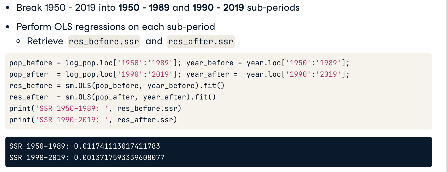
*ssr: Sum of squared (whitened) residuals. 残差平方和:它被用作参数选择和模型选择的最优准则。
Step3: Compute the Chow test statistic
Finally, we compute the Chow test statistic using the three sum of squared residuals and the degrees of freedom of the test. The Chow test statistic should be distributed as an “F” distribution. The “F” distribution has two degrees of freedom:
- The first (used in the numerator) is the number of regression parameters, here equal to 2: the intercept and slope coefficient.
- The second (used in the denominator), is the total number of data points, 70, minus twice the first degree of freedom, or 70 minus 4, which is 66.
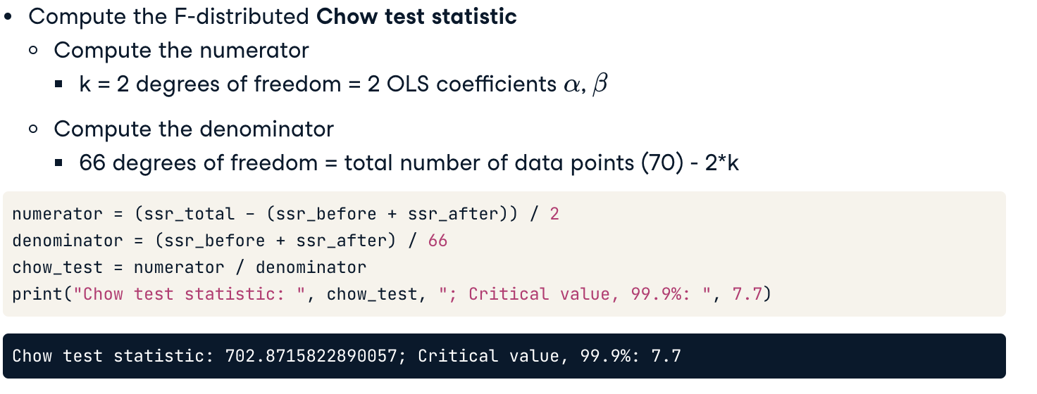
The computed test statistic is statistically different from zero at the 99.9% confidence level. We can reject the null hypothesis that there was no structural break in the data.
Exercises
Crisis structural break I
Step 1: Investigate whether something “structural” changed between 2005 and 2010.1
2
3
4
5
6
7
8
9# Create a plot of quarterly minimum portfolio returns
plt.plot(port_q_min, label="Quarterly minimum return")
# Create a plot of quarterly mean volatility
plt.plot(vol_q_mean, label="Quarterly mean volatility")
# Create legend and plot
plt.legend()
plt.show()
Crisis structural break II
Step 2: Use the richer factor model relationship between portfolio returns and mortgage delinquencies from Chapter 1 to test for a structural break around 2008, by computing the Chow test statistic for the factor model.
1 | # Import the statsmodels API to be able to run regressions |
结果1
Sum-of-squared residuals, 2005-2010: 0.05039331102490134
Crisis structural break III
Step 3: put everything together to perform the Chow test.1
2
3
4
5
6
7
8
9
10
11
12
13
14
15# Add intercept constants to each sub-period 'before' and 'after'
before_with_intercept = sm.add_constant(before['mort_del'])
after_with_intercept = sm.add_constant(after['mort_del'])
# Fit OLS regressions to each sub-period
r_b = sm.OLS(before['returns'], before_with_intercept).fit()
r_a = sm.OLS(after['returns'], after_with_intercept).fit()
# Get sum-of-squared residuals for both regressions
ssr_before = r_b.ssr
ssr_after = r_a.ssr
# Compute and display the Chow test statistic
numerator = ((ssr_total - (ssr_before + ssr_after)) / 2)
denominator = ((ssr_before + ssr_after) / (24 - 4))
print("Chow test statistic: ", numerator / denominator)
结果1
Chow test statistic: 28.93147360547482
Volatility and extreme values
Structural break indications
- Visualization of trend may not indicate break point
- Alternatively: examine volatility rather than trend
1. Rolling window volatility
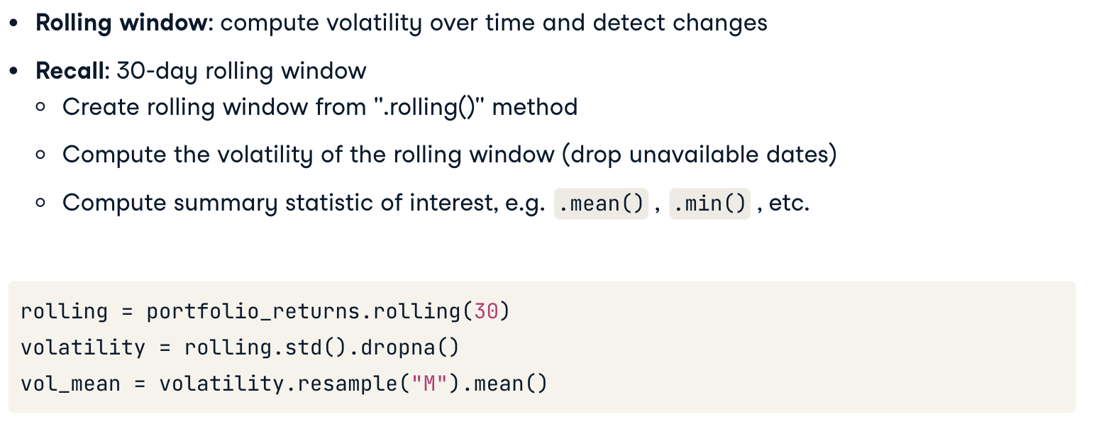
We can see if volatility is non-stationary by constructing a rolling window of losses (or returns) and computing the volatility for each window.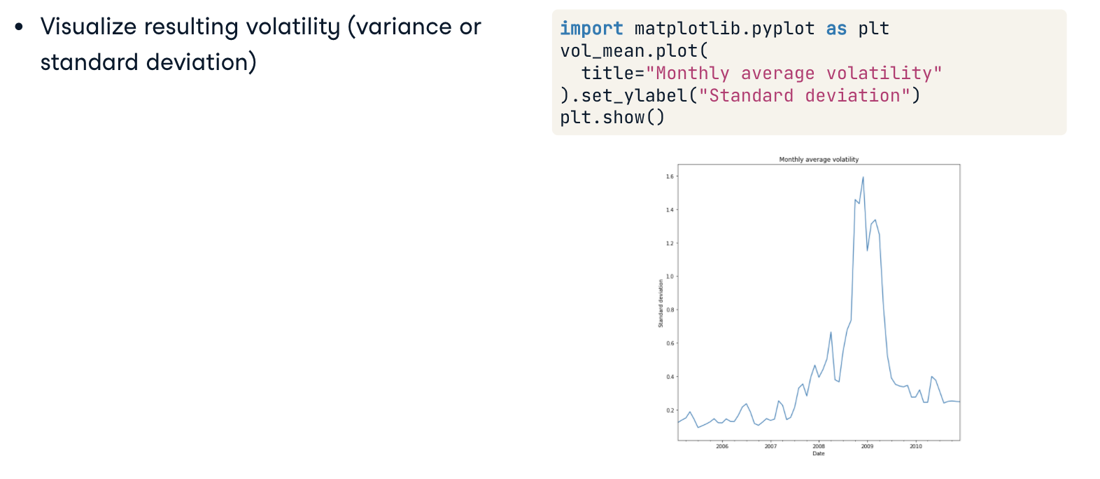
Plotting the resulting volatility series can help identify dates where the volatility appeared to change significantly. These can then be used with the Chow Test to see if one or more structural breaks is supported by the data.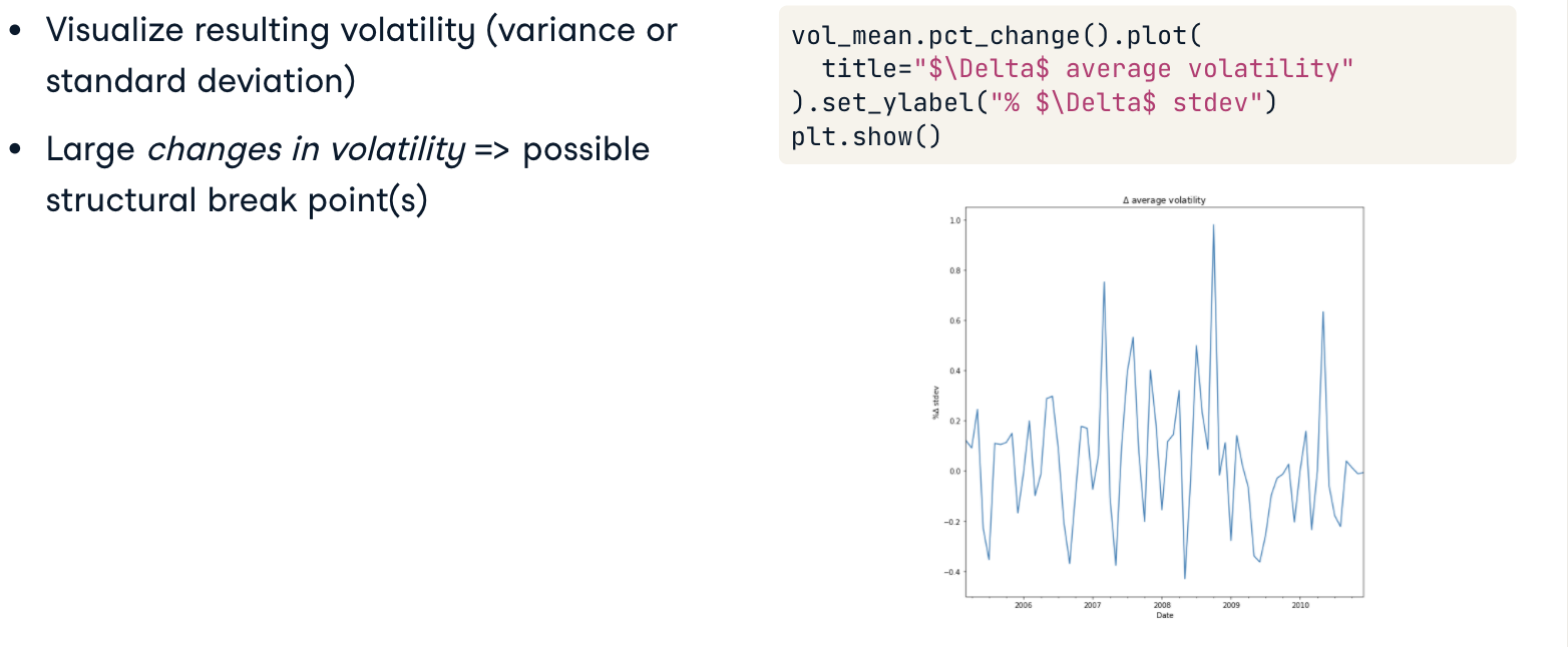
It is sometimes also helpful to visualize changes in volatility, rather than volatility itself. This provides, in addition to possible structural break points, useful information about how the variance has changed over time.
2. Extreme values
VaR, CVaR: maximum loss, expected shortfall at particular confidence level
Visualizing changes in maximum loss by plotting VaR?
- Useful for large data sets
- Small data sets: not enough information
Alternative: find losses exceding some threshold (阀值)
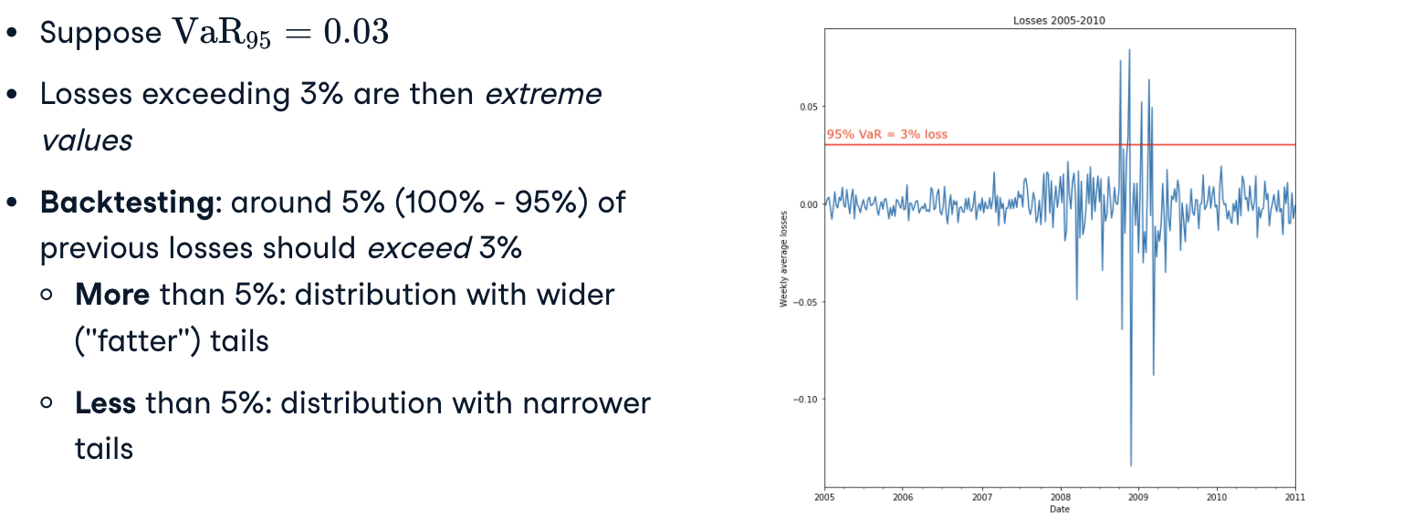
Example:VaR95 is the maximum loss in 95% of the time —> 5% of the time, losses can be expected to exceed VaR_95
Backtesting: use previous data ex-post to see how risk estimate performs
—- Used extensively in enterprise risk management
Backtesting (回测)
CVaR for backtesting: accounts for tail better than VaR
- 尾端风险/极端风险(Tail Risk)是指统计学上两个极端值可能出现的风险
- 肥尾效应(Fat tail)是指极端行情发生的机率增加,可能因为发生一些不寻常的事件
Exercises:
Volatility and structural breaks
Visualizing volatility changes helps reveal possible structural break points in time series.
By identifying when volatility appears to change, an informed choice of break point can be made that can, in turn, be used for further statistical analysis (such as the Chow test).
1 | # Find the time series of returns with and without Citibank |
Extreme values and backtesting
1 | # Compute the 95% VaR on 2009-2010 losses |
结果1
VaR_95: 0.04986983664383684 ; Backtest: 0.06547619047619048