4/4 Objectives:
- explore more general risk management tools. These advanced techniques are pivotal when attempting to understand extreme events, such as losses incurred during the financial crisis, and complicated loss distributions which may defy traditional estimation techniques.
- discover how neural networks can be implemented to approximate loss distributions and conduct real-time portfolio optimization.
Extreme value theory
Extreme value theory uses statistics to help understand the distribution of extreme values. In other words, it is a way to help model _the tail_ of the loss distribution. One way to do this is called the “block maxima” approach.
Extreme value theory: statistical distribution of extre values
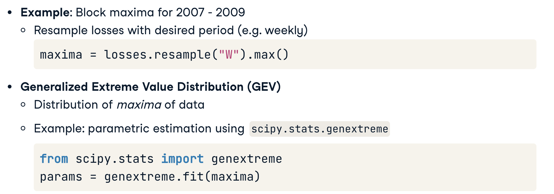
Block Maxima:
- break period into sub-periods
- form blocks from each sub-period
- set of block maxima = dataset
Peak over threshold (POT): - Find all losses over given level
- Set of such losses = dataset
Generalized Extreme Value Distribution (GEV)
VaR and CVaR from GEV distribution
Coving losses
risk management: covering losses
- regulatory requirement (banks, insurance)
- reserves must be avaliable to cover losses (for a specific time peroid/ at a specific confidence level)
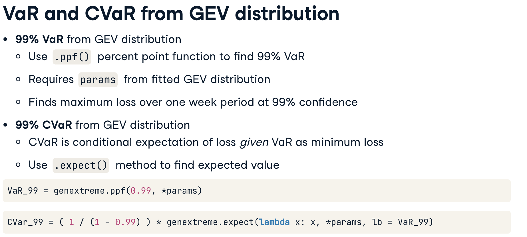
VaR from GEV distribution:
estimate maximum loss in a given period and at a given confidence level
Example: reserve requirement (储备金要求)
99%的置信水平和一周的时间范围内
Exercises
Block maxima
1 | # Resample the data into weekly blocks |
Extreme events during the crisis
1 | # Plot the log daily losses of GE over the period 2007-2009 |
1 | # Fit extreme distribution to weekly maximum of losses |
GEV risk estimation
1 | # Compute the weekly block maxima for GE's stock |
结果1
Reserve amount: 148202.41307731598
Kernel density estimation
The histogram revisited
Up to now our risk factor distributions have been assumed (such as the _Normal_ or _T distribution_), fitted (from, for example, _parametric estimation_ or _Monte Carlo simulation_), or ignored (as with _historical simulation_).
In each case, actual data can be summarized with a histogram. A histogram is not a distribution: but we would like a function to represent the histogram as a probability distribution (or density function).
How can we do this? A middle ground between parametric estimation and ignoring the distribution is to _filter the data so that they become smooth enough to represent a distribution._ This can be done with non-parametric estimation, which does not assume a parametrized class of distributions (such as the Normal, Skewed Normal, or Student’s t-distribution).
Data smoothing
Kernal: filter choice/ the “window”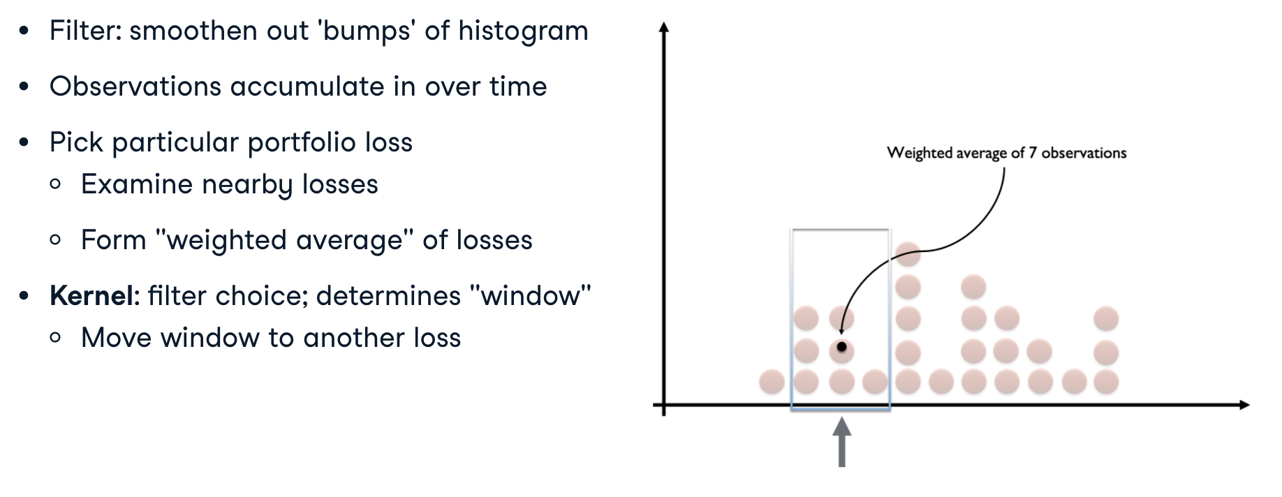
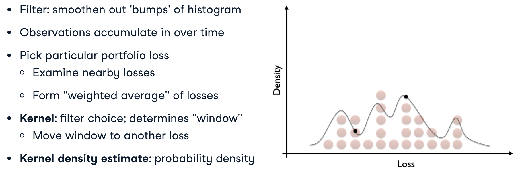
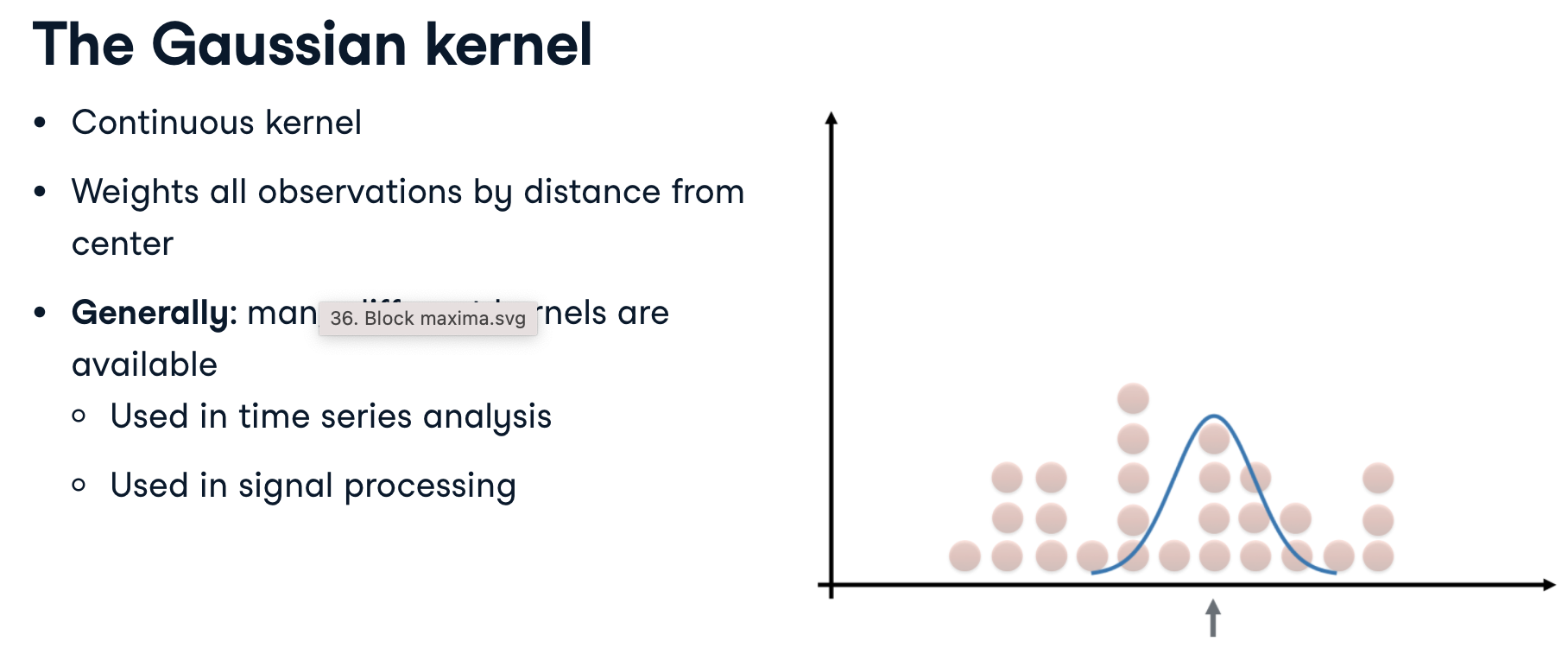
The Gaussian kernel
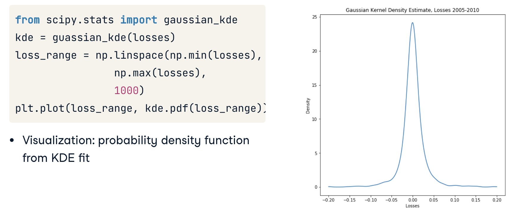
KDE in Python
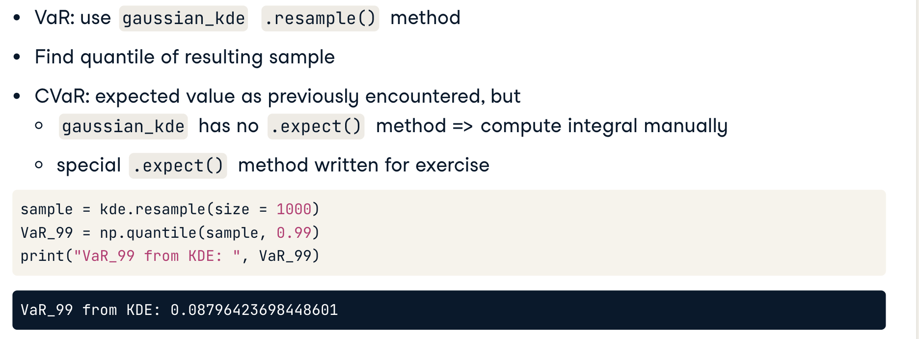
Find VaR using KDE
Exercises
1 | # Generate a fitted T distribution over losses |
Fitted distributions
- The Gaussian KDE captures the tails well, but another distribution is better at fitting the loss distribution’s peak.
- The T distribution does capture the peak well. But there’s another distribution which captures the tails of the distribution better.
- The T and Gaussian KDE estimates are both good fits, each in a different way: the T captures the peak well, while the KDE captures the tails better.
CVaR and loos cover selection
1 | # Find the VaR as a quantile of random samples from the distributions |
结果1
99% CVaR for T: 0.2716201587142073 ; 99% CVaR for KDE: 0.2395800993943245
Neural network risk management
Real-time portfolio updating
Risk management
- Define risk measures (VaR, CVaR)
- Estimate risk measures (parameteric, historical, Monte Carlo)
- Optimized portfolio (e.g. Mordern Portfolio Theory)
New Market information -> update portfolio weights
- Problem: portfolio optimization costly
- Solution: weights = f(weights)
- Evaluate f in real-time
- Update f only occasionally
Neural Networks
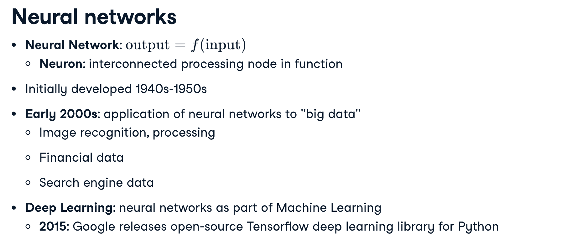
A neural network is a function: it takes an input (such as _asset prices_) and returns an output (such as _portfolio weights_).
It’s called a neural network because it contains interconnected processing nodes known as ‘neurons’, loosely resembling the connections between neurons in the brain.
Neural networks have been around since the 1940s, but they have enjoyed a resurgence of development since the early 2000s.
They are used to solve problems with large data sets, such as image recognition, financial analysis, and search engine performance.
Very large neural networks make up “Deep Learning” and are a part of the Machine Learning discipline. In 2015, Google released Tensorflow, an open-source environment, initially in Python, for performing Deep Learning.
Neural network structure
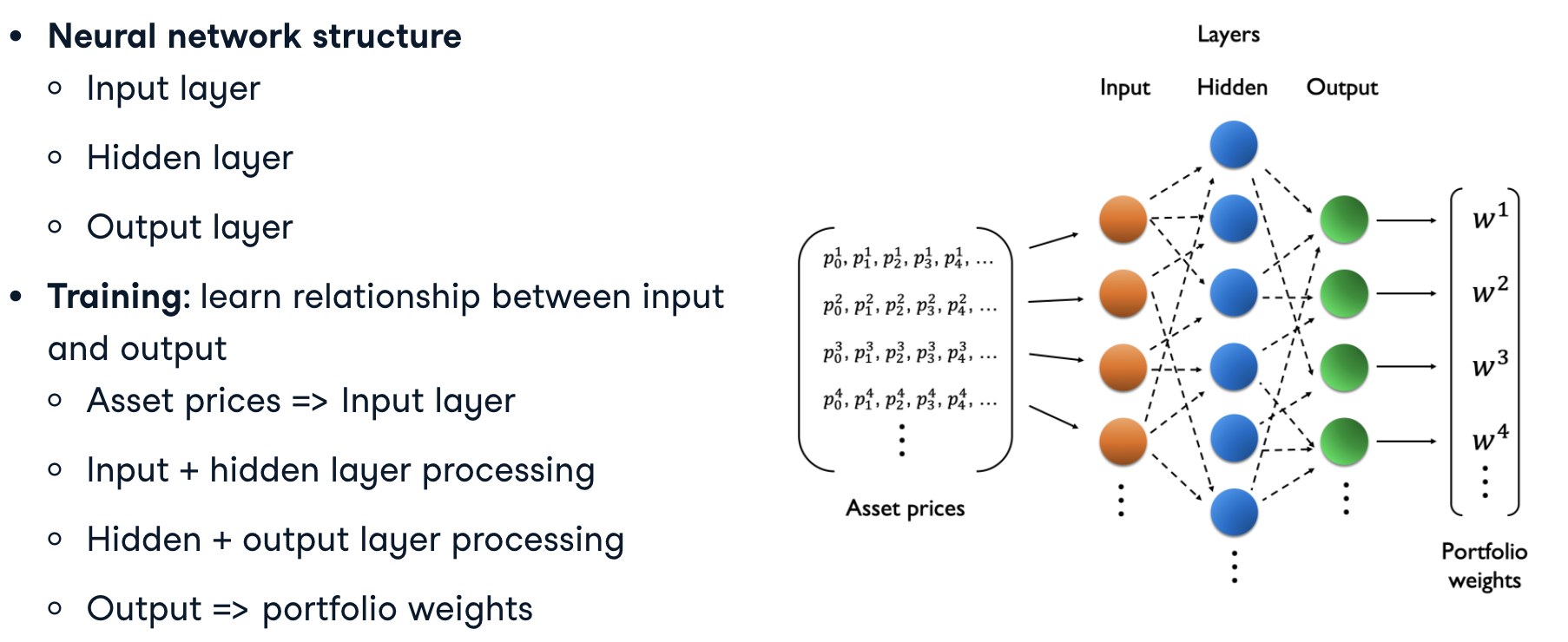
Using neural networks for portfolio optimization
Training
- Compare output and pre-existing “best” portfolio weights
- Goal: minimize “error” between output and weights
- Small error -> network is trained
通过将神经网络与预先存在的“最佳”权重进行比较,来评估神经网络在创建其输出中的表现。(这些权重可从历史数据的投资组合优化中找到)
目的是使输出和历史“最佳”权重之间的差异尽可能小,使得神经网络这个函数可以达到输出最佳投资权重的功能。
Usage
- Input: new, unseen asset prices
- Output: predicted “best” portfolio weights for new asset prices
- Best weights = risk management
Creating neural networks in Python
Keras: high-level python library for neural networks/ deep learning1
2
3
4
5from keras.models import Sequential
from keras.layers import Dense
model = Sequential()
model.add(Dense(10, imput_dim = 4, activation = 'sigmoid'))
model.add(Dense(4))
- To use Keras, we first need to import the kind of neural network—this is a ‘Sequential’ network going from input-to-hidden-to-output layers.
- Then we need to import the connections between layers (the arrows we saw previously). We’ll connect all neurons together using ‘Dense’ layers.
- Next we’ll define our neural network ‘model’ and create our hidden and output layers, using the ‘.add()’ method. Notice how the input layer is specified with the ‘input_dim’ keyword, which in our case covers the four assets in our investment bank portfolio. And since we also need four output weights, there are four “neurons” in the last output layer.
Training the network in Python
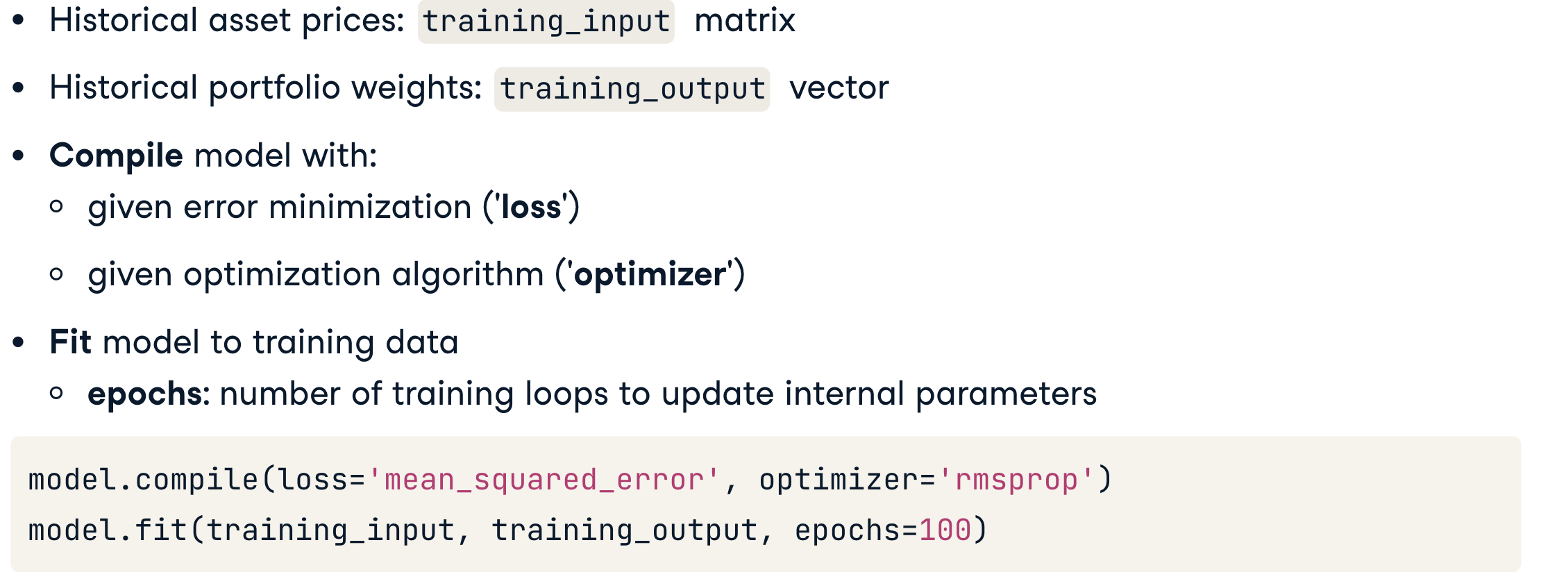
We’ve put asset prices into the ‘training_input’ matrix and portfolio weights into the ‘training_output’ vector. These are used to train the network.
- The model is first compiled to specify the error minimization function and how optimization is performed.
- Then we “fit” the network to the data, which carries out the minimization.
- The number of iterations to fit the data is given with the ‘epochs’ keyword—generally more is better.
Risk Management in Python
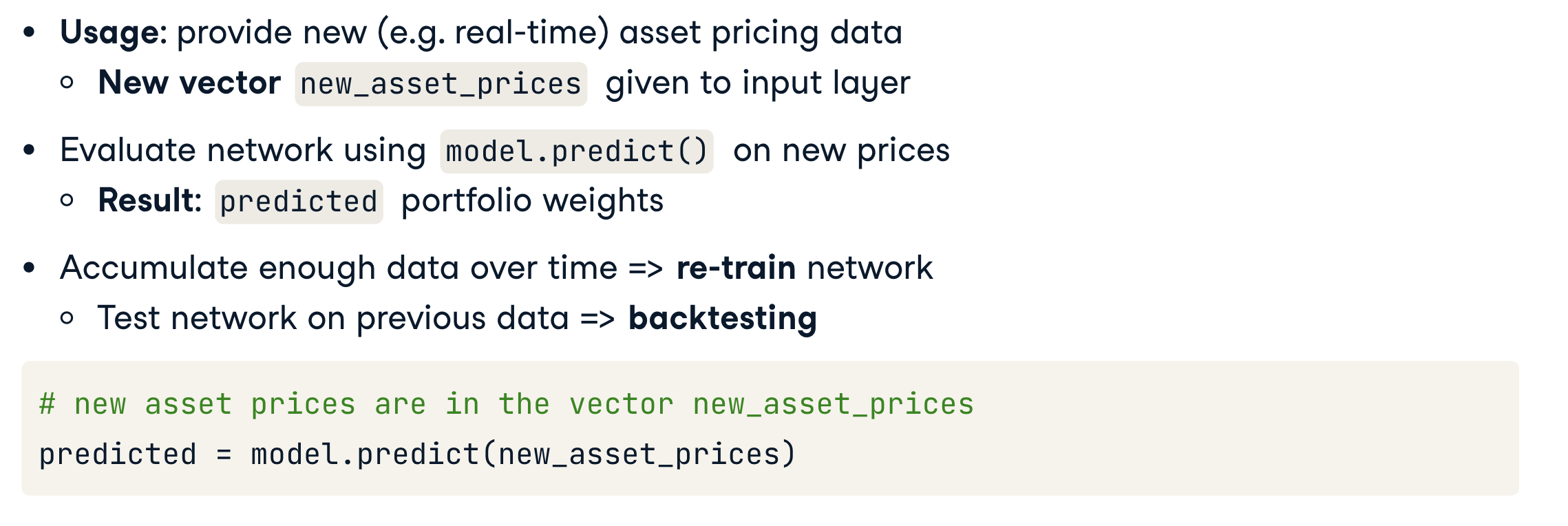
To use the network we can give it ‘new_asset_prices’ it has never seen before!
The network evaluates the new asset prices using the ‘.predict()’ method, and _returns a set of portfolio weights_.
Over time, of course, new asset prices will accumulate, and they provide valuable information. Re-training the network every so often on new data, and backtesting it on old data, is part of the neural network workflow.
Exercises
Single layer neural networks
- Create the output training values using Numpy’s
sqrt()function. - Create the neural network with one hidden layer of 16 neurons, one input value, and one output value.
- Compile and fit the neural network on the training values, for 100 epochs
- Plot the training values (in blue) against the neural network’s predicted values.
1 | # Create the training values from the square root function |
Asset price prediction
Now we can use a neural network to predict an asset price, which is a large component of quantitative financial analysis as well as risk management.
- Set the input data to be all bank
pricesexcept Morgan Stanley, and the output data to be only Morgan Stanley’sprices. - Create a
Sequentialneural networkmodelwith twoDensehidden layers: the first with 16 neurons (and three input neurons), and the second with 8 neurons. - Add a single Dense output layer of 1 neuron to represent Morgan Stanley’s price.
- Compile the neural network, and train it by fitting the
model.
1 | # Set the input and output data |
Real-time risk management
A 14-day rolling window of asset returns provides enough data to create a time series of minimum volatility portfolios using Modern Portfolio Theory, as we saw in Chapter 2. These minimum_vol portfolio weights are the training values for a neural network. This is a (1497 x 4) matrix.
The input is the matrix of weekly average_asset_returns, corresponding to each efficient portfolio. This is a (1497 x 4) matrix.
Create a Sequential neural network with the proper input dimension and two hidden layers. Training this network would take too long, so you’ll use an available pre_trained_model of identical type to predict portfolio weights for a new asset price vector.
- Create a Sequential neural network with two hidden layers, one input layer and one output layer.
- Use the
pre_trained_modelto predict what the minimum volatility portfolio would be, when new asset dataasset_returnsis presented.
1 | # Create neural network model |
结果1
Predicted minimum volatility portfolio: [[0. 0.28107247 0. 0.7649856 ]]